A 5 min guide to hyper-parameter optimization with Optuna
- 4 minsA 5 min guide to hyper-parameter optimization with Optuna
Hyper-parameter optimization with Optuna
Finding the best hyper-parameters for your model is now a breeze.

In this post, we will take a simple functioning pytorch neural network training script and enhance it using the [Optuna](https://optuna.org/) package(docs here). This will allow easy assimilation of smart hyper-parameter tuning and trial pruning into your ML workflow with minimal code modifications.
Personally, finding the best hyper-parameters to fit my objective has been the worst part of my ML workflow. Up until now, my choices were two: (1) sacrifice my time and sanity and use good old graduate-student-descent or (2) implement a complicated framework to search the parameter space, find the best values, document and visualize the process.
The good news: such a framework already exists, it’s called Optuna, and it’s easy and fun to use.
Our starting point is an MNIST classification script from the Pytorch tutorials. The full script is presented here for completeness, however, since none of the other parts are relevant to our point, I recommend skimming through all parts leading up to the main function.
If you want to see the code in action, below is a link to a working google colab notebook. Google Colaboratory Optuna MNIST pytorch
Now let’s get down to business.
Vanilla MNIST Classifier Framework
We begin with imports and data loaders:
Next, we implement the network:
The train and test methods:
And the main function:
Notice that up to this point, nothing interesting really happened, just a simplified pytorch MNIST classifier script. Training the above script with the current randomly chosen hyper-parameters for 5 epochs will give 93% accuracy. Can we do better? Let us see…
Enhancing the MNIST classifier framework with Optuna
The Optuna framework (installed via pip install optunaand imported as import optuna ) is based upon the *study *object. It contains all of the information about the required parameter space, the sampler method and the pruning:
Once the study is created, the search space is incorporated via the trial.suggest_ methods. We will embed these into the train_mnist config such that these values:
will be replaced with these:
In this manner we define the search space to our requirements, once this is done, train_mnist() should get trial as its input and be defined as train_mnist(trial) . Note that a configuration which allows train_mnist to have inputs other than trial exists, check this out, if you come across this need.
Optimization
The final step is to define an objective function, the output of which will be optimized over. In our case we choose train_mnist and its output, the test error¹.
Therefore study.optimize will be called, with train_mnist as its parameter:
All in all, main, which was comprised of a single call for train_mnist() , has turned into:
And that’s it! Once these lines are added to the code, the optimizer will sample the defined parameter space according to the sampler.
After optimization is done, results can be accessed as a dataframe via study.trials_dataframe:
With the following output:
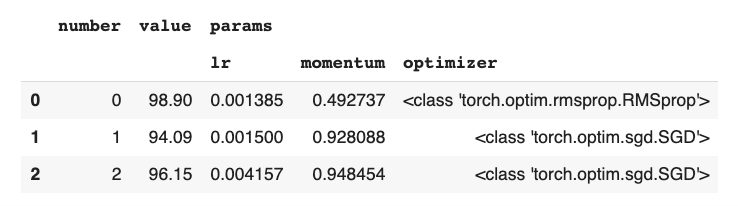
were one can see all trials and their value. To find the best trial best parameters, study.best_trial and study.best_params can be also used.
Here, we also see how one of the results got a 98.9% test error (~6% improvement) with the same amount of training data and time, this is a major improvement for 3 lines of code.
Visualization
Other than showing you the best configuration of parameters, Optuna also helps in visualizing the dependence of the objectives on the parameters. Given the study object, all sorts of visualization tools exist in optuna.visualization . You can call plot_parallel_coordinates(study) to view the dependence between the parameters (in this case- lr and momentum) and the objective:

Another way to try to gain some intuition is by using a contour plot. This can be produced by calling plot_contour(study) :

To complete the picture, you can also produce a slice plot by calling slice_plot(study) . This can help with the understanding of where the best subspaces are located for each parameter individually.

One last visualization option is the study history, produced by plot_optimization_history(study) . This will present the following plot:

This shows how Optuna’s study takes place, first by sampling the space evenly, then by focusing in on the most promising areas.
To conclude, I hope you enjoyed this tutorial, I left out several great features like early pruning and different search algorithms, which will have to wait for another time. If I’ve piqued your interest, check out the great Optuna documentation, it’s all there.
Enjoy!
[1] Note that in this article I perform a terrible crime for the sake of brevity: one should never optimize over the test set, as it will overfit the testing data! A better path would be to split the training set into train and validate, but since this is not the subject of this post, I‘ve decided to leave it as is.